CODE
# PREPARING DATASET
library(tidyverse)
library(rio)
library(janitor)
# Load data and filter for Graduation only, but retain other classes for a balanced dataset
DataStore <- import("C:/Users/aishw/Downloads/superstore_data.csv") %>%
clean_names("upper_camel") %>%
select(NumWebVisitsMonth, NumWebPurchases, Education)
# Ensure at least one instance of each education level is included
DataStore <- DataStore %>%
filter(Education %in% c("Graduation", "Basic", "Master", "PhD")) # Keep more classes for analysis
head(DataStore)
OUTPUT
EXPLANATION
The head(DataStore) function in R is used to display the first few rows of a data frame. It provides a quick overview of the data structure, column names, and sample values.
In the context of your code, DataStore is a data frame containing information about the number of web visits, number of web purchases, and education level for a set of individuals. The head(DataStore) function will print the first few rows of this data frame, showing you the values for these variables in the first few observations.
CODE
# SPLIT DATASET
library(tidymodels)
set.seed(876)
# Splitting the data, ensuring there are enough samples for the KNN model
Split7030 <- initial_split(DataStore, prop = 0.7, strata = Education)
DataTrain <- training(Split7030)
DataTest <- testing(Split7030)
print(DataTrain)
print(DataTest)
OUTPUT
EXPLANATION
The code in the image is splitting a dataset into training and testing sets for machine learning.
1. initial_split(DataStore, prop = 0.7, strata = Education):
- Splits the dataset
DataStore into training and testing sets. prop = 0.7 specifies that 70% of the data will go to the training set, and 30% to the testing set.strata = Education ensures that the proportion of each education level is similar in both sets, preventing bias.
2. training(Split7030) and testing(Split7030):
- Extracts the training and testing sets from the split.
DataTrain contains 70% of the data, and DataTest contains 30%.
3. print(DataTrain) and print(DataTest):
- Prints the first few rows of the training and testing sets for inspection.
This code is preparing the data for modeling by creating separate sets for training the model and evaluating its performance on unseen data.
CODE
# KNN
RecipeStore <- recipe(Education ~ NumWebVisitsMonth + NumWebPurchases, data = DataTrain) %>%
step_naomit() %>%
step_normalize(all_predictors())
print(RecipeStore)
# CREATING A MODEL DESIGN
ModelDesignKNN <- nearest_neighbor(neighbors = 4, weight_func = "rectangular") %>%
set_engine("kknn") %>%
set_mode("classification")
print(ModelDesignKNN)
# RUNNING KNN
WFModelStore <- workflow() %>%
add_recipe(RecipeStore) %>%
add_model(ModelDesignKNN) %>%
fit(DataTrain)
print(WFModelStore)
# PREDICTING
# Make predictions on the test data
predictions <- predict(WFModelStore, DataTest) %>%
bind_cols(DataTest)
OUTPUT
EXPLANATION
It preprocesses the data, defines the model parameters, trains the model on the training data, and makes predictions on the testing data.
CODE
# Convert predicted and true labels to factors
predictions <- predictions %>%
mutate(
Education = as.factor(Education),
.pred_class = factor(.pred_class, levels = levels(Education))
)
# Display first few rows of predictions with test data
head(predictions)
# CONFUSION MATRIX
# Print confusion matrix
confusion_matrix <- conf_mat(predictions, truth = Education, estimate = .pred_class)
print(confusion_matrix)
OUTPUT
EXPLANATION
The above code prints the confusion matrix.
CODE
# ACCURACY
library(yardstick)
# Calculate accuracy
accuracy_result <- accuracy(predictions, truth = Education, estimate = .pred_class)
print(accuracy_result)
# Calculate sensitivity
sensitivity_result <- sensitivity_vec(predictions$Education, predictions$.pred_class)
print(sensitivity_result)
# Calculate specificity
specificity_result <- specificity_vec(predictions$Education, predictions$.pred_class)
print(specificity_result)
OUTPUT
EXPLANATION
The above code calculates accuracy specificity, sensitivity, and accuracy.
CODE
# PLOTTING GRAPHS
# Plot confusion matrix using ggplot2
library(ggplot2)
print_confusion_matrix <- function(cm) {
cm_table <- as.data.frame(cm$table)
cm_wide <- cm_table %>%
spread(key = Prediction, value = Freq, fill = 0)
# Use actual class labels from confusion matrix
cm_matrix <- as.matrix(cm_wide[, -1])
rownames(cm_matrix) <- cm$reference
# Print the confusion matrix
print(cm_matrix)
}
# Plot accuracy, sensitivity, and specificity
metrics <- tibble(
Metric = c("Accuracy", "Sensitivity", "Specificity"),
Value = c(accuracy_result$.estimate, sensitivity_result, specificity_result)
)
ggplot(metrics, aes(x = Metric, y = Value, fill = Metric)) +
geom_bar(stat = "identity") +
theme_minimal() +
labs(title = "Model Metrics", x = "Metric", y = "Value") +
ylim(0, 1)
# SCATTER PLOT
# Scatter plot of predictions
ggplot(predictions, aes(x = NumWebVisitsMonth, y = NumWebPurchases, color = .pred_class, shape = Education)) +
geom_point(size = 3) +
theme_minimal() +
labs(title = "Scatter Plot of KNN Predictions", x = "Number of Web Visits per Month", y = "Number of Web Purchases", color = "Predicted Education Level", shape = "Actual Education Level")
OUTPUT
EXPLANATION
The above code prints the scatter plot.


Comments
Post a Comment